hpdz.net
High-Precision Deep Zoom
Technical Info - Antialiasing
Introduction
This page describes the problem of aliasing in rendering fractal images and examines some ways to mitigate its effects. This always involves doing things that dramatically increase the rendering time of the fractal, so for many deep-zoom animations, it is not practical to use any of these methods unless frame interpolation is used.
This page has the following topics:
- Some DSP Theory
- Aliasing
- Anti-aliasing
- How Much Supersampling?
- Filtering
- Selective Supersampling
- Conclusions
The related subject stochastic supersampling is discussed on a separate page.
Some DSP Theory
Digital signal processing is a branch of electrical engineering and mathematics that deals with signals that have been digitally sampled and are processed as discrete lists or arrays of numbers, as opposed to analog signals. Most of this field was originally developed to understand the processing of audio signals that are digitally sampled in time, but it turns out that essentially the same mathematics applies to images that are digitally sampled in a two-dimensional plane. Obviously all fractal images rendered by software that scans a region of the complex number plane are digitally sampled, so DSP has a lot of important insights regarding this business.
The most important result to understand is the Nyquist-Shannon sampling theorem:
If a signal y(t) contains no frequencies higher than F0, then it can be completely reconstructed by sampling at a frequency F > 2F0, by a grid of sample points spaced at intervals of dt = 1/F < 1/(2F0).
This can be restated slightly differently for two-dimensional images:
If an image A{x,y} contains no spatial detail on scales smaller than size ds, then it can be completely reconstructed by sampling on a grid of points spaced at intervals smaller than dx=ds/2 and dy=ds/2.
The frequency 2F0 is called the Nyquist frequency. The requirement that a signal have no energy at frequencies higher than F0 is called the Nyquist criterion. Note that the Nyquist frequency is twice the limiting frequency F0.
As important as this theorem is for providing guidance on how to reconstruct sampled signals, it is also important for fractal animations because it tells us what we cannot do: we cannot hope to reconstruct the fractal by sampling on a grid because the fractal always has spatial detail smaller than any distance scale ds that we can choose. This is a fundamentally different situation than electrical engineers face when sampling analog signals.
Normally, when an analog signal is digitally sampled, it is first run through a low-pass filter that removes energy in the signal above the frequency F0. Although it may not be easy, it is at least possible in principle to filter an analog signal well enough to achieve any desired level of attenuation of the signals at frequencies higher than F0, and the Nyquist criterion can be satisfied well enough for most practical purposes (even enough to make the fussiest audiophiles happy).
The same principle applies to images. Digital cameras, for example, have to employ the optical equivalent of a low-pass filter before the image gets to the digital image sensor. In this case, the low-pass filter is an optical element that blurs the image very slightly to ensure that there is no detail on scales smaller than twice the image sensor's pixel spacing.
Unfortunately, there is no way to do something analogous when we try to draw a fractal. No matter what we do, we are always beginning with the sampling operation -- there is no way to insert a low-pass filter in the image before we sample it. The phenomenon that happens when we digitally sample a signal without first filtering out the energy above the Nyquist frequency is called aliasing.
Aliasing
If we go ahead and sample a signal with significant energy above F0, it turns out that all the energy above F0 gets folded back into the frequency range below F0. This is called "aliasing" because when the digitally sampled signal is reconstructed from its samples, high frequency input signals will be converted to some other, lower frequency; it is as if the high frequency took on a new identity as a lower frequency. This is the same phenomenon that makes it look like car wheels are moving slowly (or backwards) when you watch them on TV or a movie.
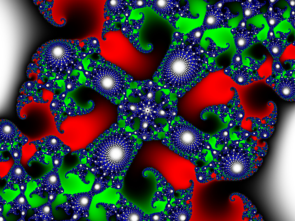
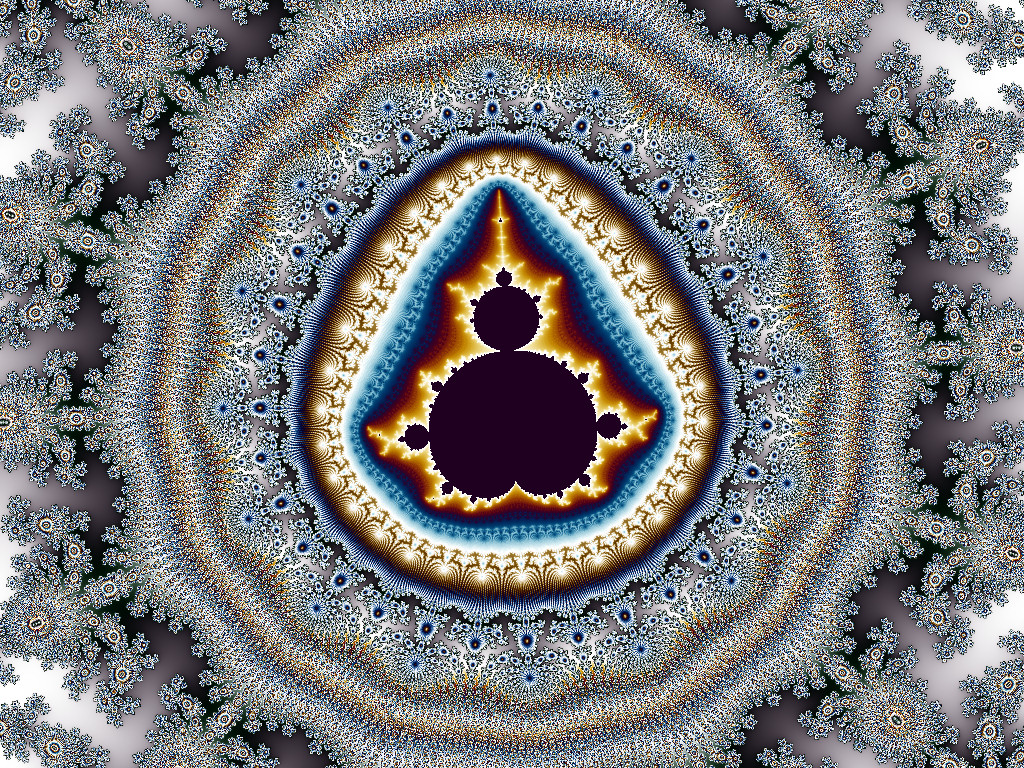
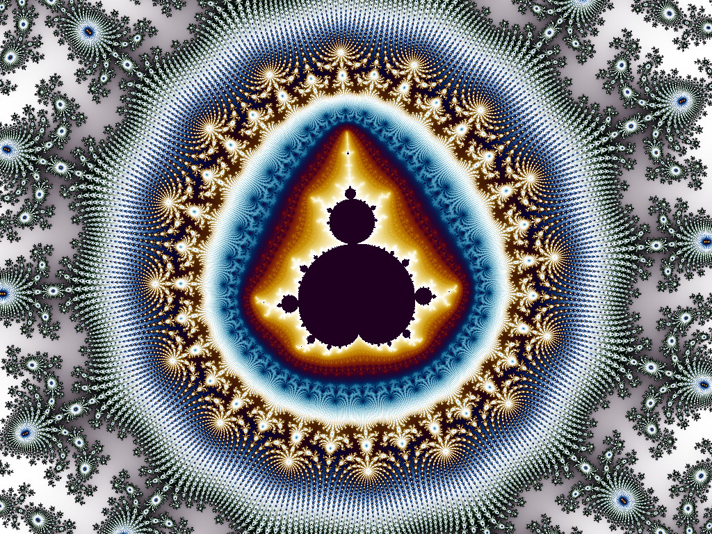
In fractal animations, this effect is most obvious in areas with lots of extremely fine spatial detail, and manifests as formation of moire patterns. Here is an example, taken from the video Centanimus, with a size of about 1e-100 (click for a larger version):
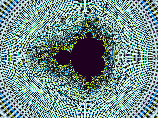
When the spatial frequency of the fine radial spokes converging on this mini-set's edge becomes higher than the Nyquist frequency determined by the spacing of the sampling grid, aliasing starts to happen. The high frequencies get aliased to low frequencies, which manifest as the moire patterns we see. These generally don't show up except at extreme deep-zooms like this where there is a tremendous amount of detail on exquisitely small scales compared to the pixel size.
In the image above, when we look at the area right next to the set, all we see is noise. This is because the spatial frequencies of the converging radial lines are so high that they get folded back many times into the spatial frequency band below F0. That multiple folding effectively scrambles all the information in this region, and what we see is just noise. So we can think of each mini-set (and remember there are infinitely many of them) as surrounded by a little cloud of noise with very high spatial frequency. Furthermore, since the count numbers rise arbitrarily high as we get closer to the boundary of a set, and are indeed infinite within the set itself, the amplitude of the noise in this cloud can be arbitrarily large.
This is what causes the "sparkle" noise effect that can be seen to some degree in all fractal animations.
Anti-Aliasing
Although it is impossible to eliminate the effects of aliasing altogether, there are ways to reduce them or make them less visible.
Fundamental Rules
A very deeply-rooted fact (not a theoretical proposition) is that there are only two ways to deal with aliasing:
- Prefilter the signal to remove as much of the energy above the Nyquist limit as necessary
- Oversample the signal at a rate well above the Nyquist frequency
Maybe the more laid-back people would add another choice:
- Ignore it (or even enjoy it!)
Fractal images (and indeed, all digital video images that are constructed from mathematical models, including things like Shrek and Nemo) do not exist until they are digitally sampled; there is nothing analogous to prefiltering an analog signal in the world of computer graphic imaging, so option (1) is not available.
Therefore, all anti-aliasing techniques for fractal images, whether still or animated, are variations on one fundamental idea, which is oversampling (another synonymous term is "supersampling" which I like because it sounds more cool).
Overampling
Oversampling refers to sampling a signal at a rate much higher than the maximum frequency that needs to be reproduced. In the case of fractal images, it means sampling the fractal on a grid with many more pixels than the final image contains. For example, we could use a 3x3 grid, or a 5-point cross, or even just two points next to each other (or the tricky technique of stochastic supersampling).
What this does is increase the sampling frequency, which means the the same amount of aliased energy will be spread over a much larger signal bandwidth. That means the energy density of the aliased energy will be lower in the signal band.
Another way of thinking of this is that the aliased energy is spread into some discrete frequency bins, whose number is half the number of sample points. Increasing the number of sample points increases the number of frequency bins, but the amount of out-of-band energy that will be aliased is the same, so the aliased energy per bin is lower.
Any sampling also establishes an absolute limit to the frequency content of the signal -- once any signal is sampled at a rate F, it cannot reproduce any frequency content above F/2. So if the oversampled signal is low-pass filtered and then sampled again -- this time with the Nyquist criterion more closely satisfied, since the oversampled signal can be low-pass filtered -- the amount of aliased noise in the final reproduced signal is lower.
What that translates to in practical terms is that we calculate the fractal on a much larger grid than we really need, with the pixels on that larger grid spaced more closely than the pixels will be in the final image. The finer-spaced pixels give a higher sampling frequency. We then apply a low-pass filter of some sort (which type of filter is a whole subject in itself) to the oversampled grid and resample the output of that filter at the spatial resolution of the final video image.
Bottom Line
So all techniques for reducing noise in computer-generated fractal images are basically variations of oversampling and low-pass filtering. The most obvious questions now are:
- What kind of filter do we use?
- How much oversampling do we need?
There is also a more subtle question about how to oversample...more on that later.
How Much Supersampling?
The second question turns out to be the more important one, and its answer is easy: The more the better. Well, up to a point.
The effects of oversampling follow one of the general rules of life, the Law of Diminishing Returns. A few extra points of oversampling, like 2X in each direction (for a total of 4X the number of points) gives a significant effect, while going to 3X gives a little more effect but not as much, and going to 4X gives an even smaller improvement. Generally, oversampling beyond 5X (25 samples per output pixel) doesn't give enough of a noticeable improvement to justify the 25X increase in rendering time. The histograms and sample images below -- some of which are drawn with 15x15 oversampling -- show this quite clearly.
Filtering
The first question above -- what type of filter to use -- is more difficult. There are dozens of different kinds of digital filters, many of which have dozens of variations, and many of which allow some sort of multi-parameter kernel to be specified... Broadly speaking, they are divided into two major groups; linear filters and nonlinear filters. We are not going to go into any details of this, but rather consider one simple linear filter, the mean filter, and one simple nonlinear filter, the median filter.
The median filter turns out to be superior for our purpose, as we will see with the test images below. Still, the difference between these filters is often quite subtle, especially when compared to the impact of having more oversampling points. But it is possible that there are other more sophisticated filters that we could use. This is an ongoing area of interest in the research department of HPDZ.NET, and some developments may come in the future.
Mean Filter
One obvious thing to do when we have a bunch of data samples and want to reduce them to a single number is simply take their average. If we just take each image pixel and divide it into a small grid for oversampling, we can average those oversampled points together and use the average in the final video frame.
This turns out to work fairly well, as shown by the test images below. Click on the thumbnails to download the 1024x768 JPG files. The JPG compression is set very low on all these files to preserve detail as much as possible, so they are all pretty big, around 700-900KB each.
 |
 |
||
| Unfiltered | 5x5 | ||
 |
 |
 |
|
| Unfiltered | 3x3 | 15x15 | |
 |
 |
 |
 |
| Unfiltered | 15x15 | Unfiltered 2 cycles |
15x15 2 cycles |
About the Example Images
- The first row was used to make some of the example histogram plots below. The images are drawn with max counts = 100,000 and rank-order colorizing is used.
- The second row is taken from the examples comparing histogram versus rank-order colorizing and uses histogram colorizing.
- The third row is an area chosen for its high level of detail. It was drawn with rank-order colorizing with max counts = 100,000 and includes examples with a 2-cycle color palette.
The results are pretty good, but this is not the optimal filter for this application. That is because the mean of a set of data gives a lot of weight to outlier values and doesn't always produce the result we want when the data has a single large, spurious value. Say we have a 3x3 oversampling grid that has fractal count values as shown below in set S. This kind of data is typical of what we see in the Mandelbrot set, with occasional huge spikes that we want to remove from the count values.
S = { 90, 101, 110, 120, 126, 150, 173, 182, 10000 }
The average of the values in S is 1228. This value is not really representative of the data set in this case. Furthermore, the average is not one of the members of the original input data set. That means that this kind of filter will introduce count values into the fractal image that were not calculated at any point in the supersampling grid.
The mean filter is very good -- optimal, in fact -- at removing a certain type of noise, namely Gaussian-distributed noise, but it is not so good at removing the kind of spiky, impulsive noise that we have in this application.
Median Filter
Another way to reduce a set of data to a single number is to take the median. The median of a set is the number in the set which half the data is above and half the data is below. If the set has an odd number of points, the median is the data point in the middle when the data is sorted. If the set has an even number of points then the median is the average of the two center data values.
Consider the previous data set on the hypothetical 3x3 oversampling grid.
S = { 90, 101, 110, 120, 126, 150, 173, 182, 10000 }
The median of this set is 126, which is more representative of the data than the mean of 1228. The median of a set is better able to reject large outlier values than the mean is. Notice that the median will be the same no matter how large the largest value gets, while the median will grow proportionally to the largest value. Also, notice that the median is one of the data set members, 126 in this case, while the mean value of 1228 is not an element of S. As long as the set S has an odd number of elements, the median will always be a member of S and therefore will always be a value that was actually calculated from the fractal formula, not a value that is an artifact of the filter.
In terms of the performance on images, the median filter is a much better choice for this application because median filters remove impulsive, spiky noise much more effectively than any kind of filter based on averaging. Note that we are only using the filter on the supersampling pixels; we are not filtering the final image itself.
Here are some examples of its effect on the previous test images.
|
|
 |
||
| Unfiltered | 5x5 oversampling | ||
|
|
 |
 |
|
| Unfiltered | 3x3 oversampling | 15x15 oversampling | |
|
|
 |
|
 |
| Unfiltered | 15x15 | Unfiltered 2-cycles |
15x15 2-cycles |
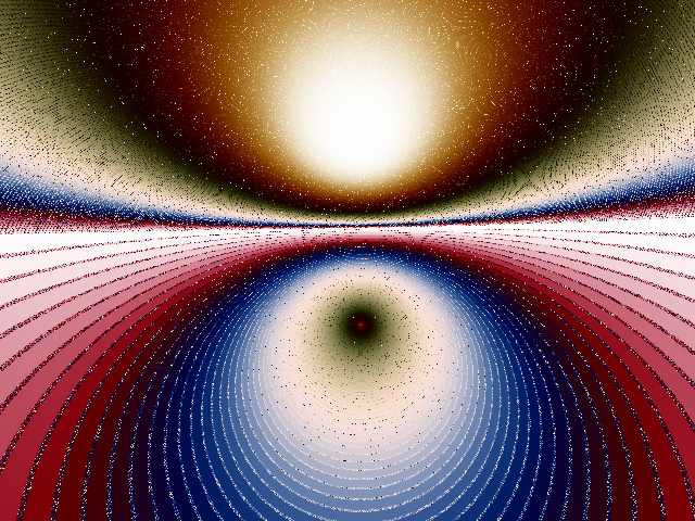
Here's a couple more examples that I made a long time ago and just had to keep. These are at a size of 1.2e-15 in the complex number plane. They show how much sparkle noise can be eliminated by supersampling and also show some subtle moire in the upper half that is diminished in the filtered version. Note that the filtered JPG file is significantly smaller than the unfiltered file since it has much less noise.
 |
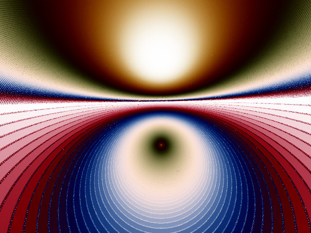 |
| Unfiltered JPEG 225KB | Filtered JPEG 140KB |
Histograms
We can gain some insight into the differences between the mean filter and median filter, as well as the effect of additional oversampling, by looking at the count histograms for images with different types of oversampling.
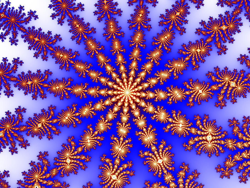
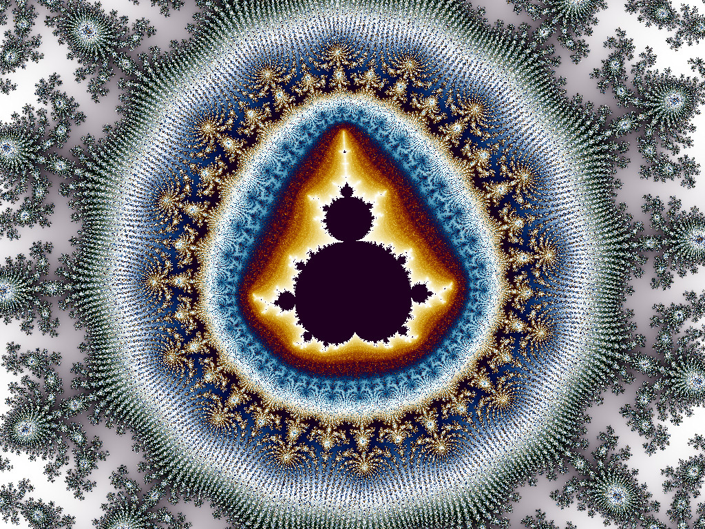
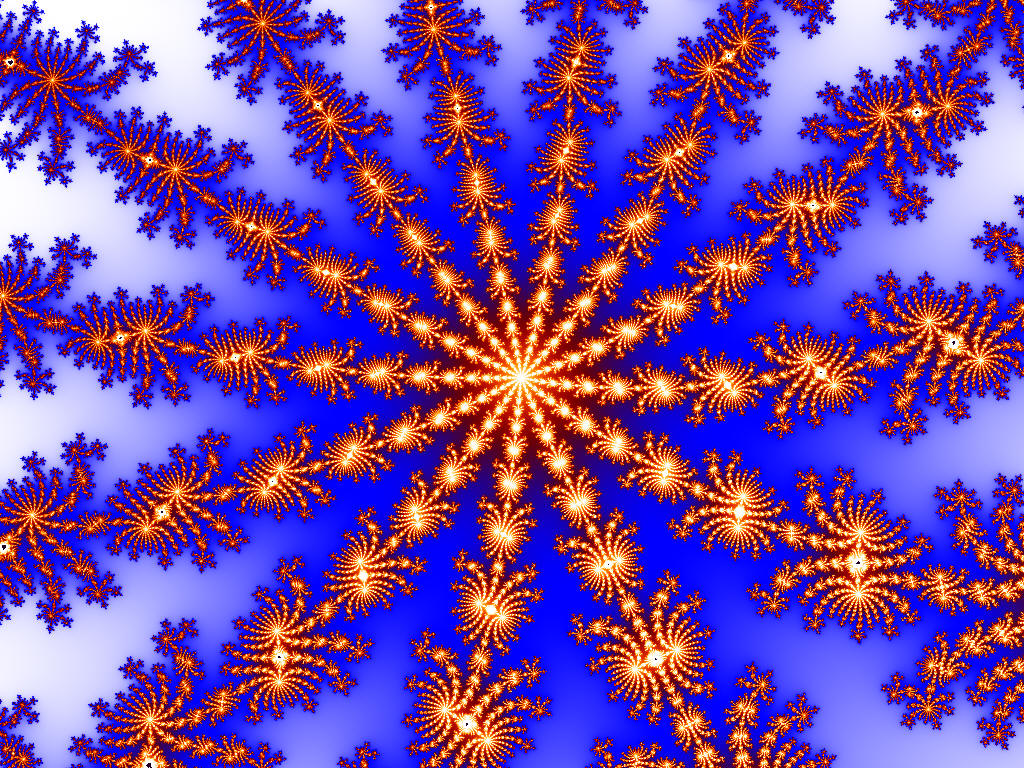
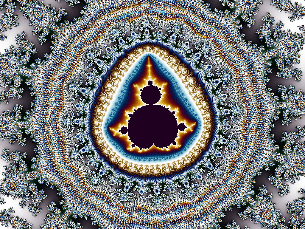
The first set of histograms comes from the image in the first row of the sample images above, the one that looks like this:

The first histogram was generated from images that were made with the maximum count number set to 500 and rendered with a resolution of 500x500 pixels. The following five configurations were used. In case the legend on the graph is not clear, the colors of each group of data are listed below.
- Unfiltered data (black)
- Median filter, 5x5 oversampling (red)
- Median filter, 15x15 oversampling (violet)
- Mean filter, 5x5 oversampling (green)
- Mean filter, 15x15 oversampling (blue)
The unfiltered data is black; the green/blue points are the mean filtered data, and the red/violet points are the median filtered data.
The histogram, which is shown in log-log scale, is a plot of the frequency of each fractal data value in the image. The horizontal axis indicates the fractal count number, on a scale from 50 to 500 (the maximum possible for this set of images). Each minor log division represents a multiple of 10, so the minor ticks correspond to 50, 100, 150, 200, etc. up to 500. The vertical axis is proportional to the number of times each number occurs in the image, scaled by an arbitrary factor to make the range look nice. It is essentially the probability density function for the counts.
The first thing to notice about this graph is that the mean-filtered points (green and blue) have a prominent hump around counts 200-250. This hump is not present in the original unfiltered data (black points) and is due to the effect described above -- the mean of a set of data with an outlier will give a value intermediate between the outlier and the true central value of the data. This hump is not present in the median-filtered (red and violet) data.
Next, notice that the mean-filtered points retain a slightly higher maximum count value than the median-filtered points. This is also because of the fact that the mean will give significant weight to outlier points and is less able to eliminate them from the data than the median can.
Finally, compare the difference between the 15x15 median filtered values (violet) and the 5x5 median-filtered value (red) to the corresponding difference for the mean filtered values. The median filter at 5x5 performs much closer to how it does at 15x15 than the mean filter does. The median filter is better able to filter out noise with fewer oversampling points than the mean filter is -- for the particular type of noise we have here. This makes a huge difference in rendering fractal images, where the difference between 5x5=25 and 15x15=225 can mean the difference between a project taking a month versus a project taking a year.
Now let's look at what happens when we raise the max count to 100,000. Remember the vertical axis has an arbitrary scale, so don't compare it with the previous graph.
This histogram has the horizontal (count) axis extended to 1000 to show the higher count numbers that occur now that the max count is 100,000 instead of 500, but there are actually a few additional points with counts well above 1000, extending to th 10,000 to 100K range. Of the several hundred thousand total points in this data set, only about ten had counts above 1000, so we've chopped them off here since they have a negligible effect on the main conclusions below. But if you are scaling based on the maximum count, these outliers can be devastating, which is why trimming (ignoring the few highest and lowest counts) is essential for colorizing.
Two important things seem to jump out:
- The humps in the mean-filtered data are more prominent. This is because there are more high-valued outliers that are artificially pulling the means up to the 200-250 range.
- The difference between the 5x5 mean and the 15x15 mean is larger, while the difference for the median filtered data is no different. Again, the median filter is much more robust, even for smaller oversampling factors, than the mean filter.
The median filter seems to be performing more like what we would want, at least based on this set of data from this particular image.
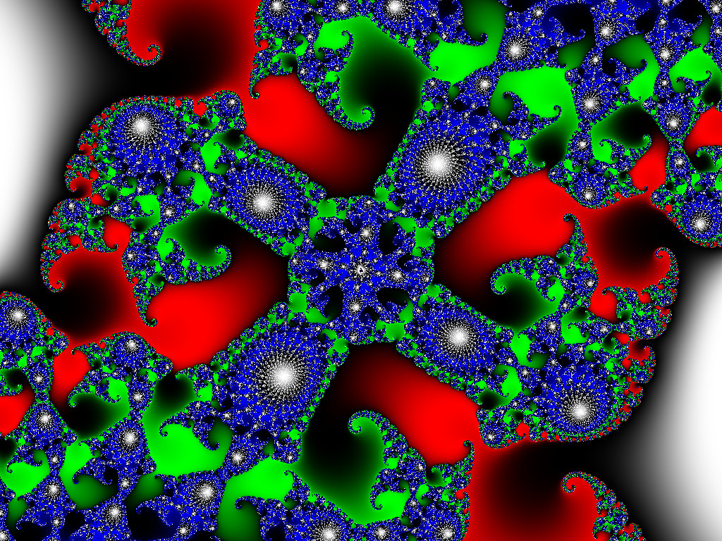
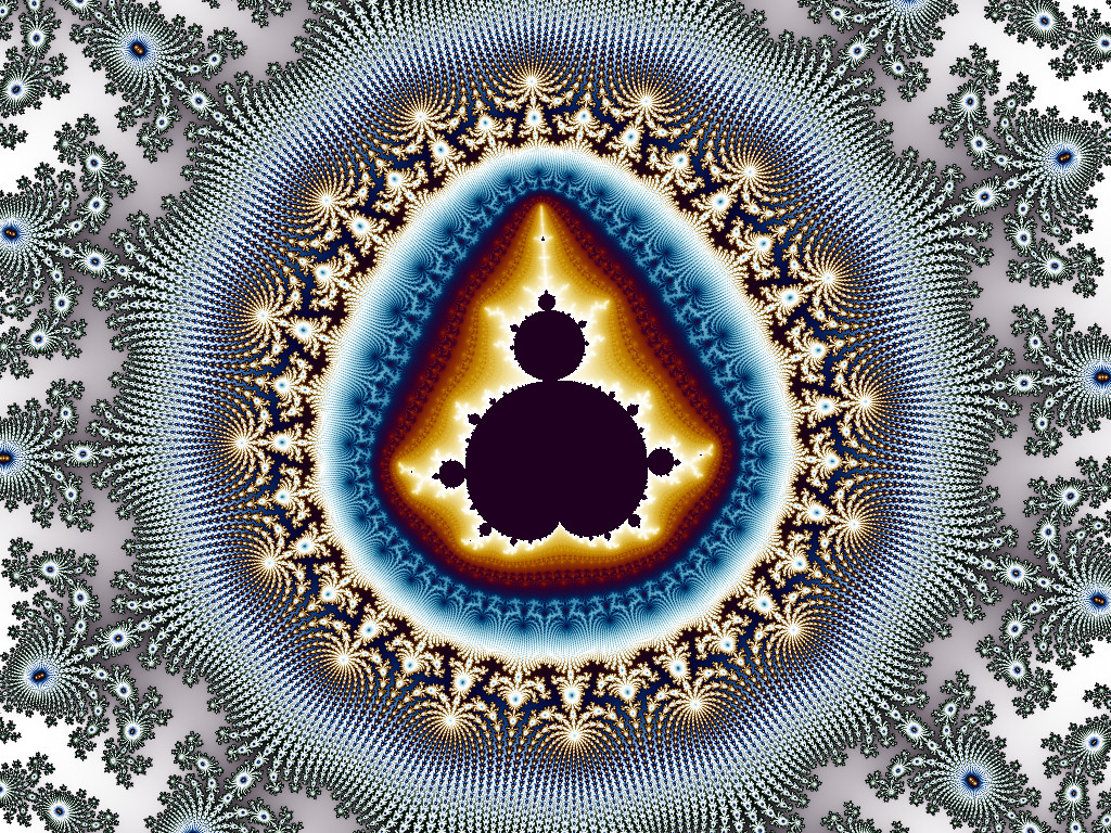
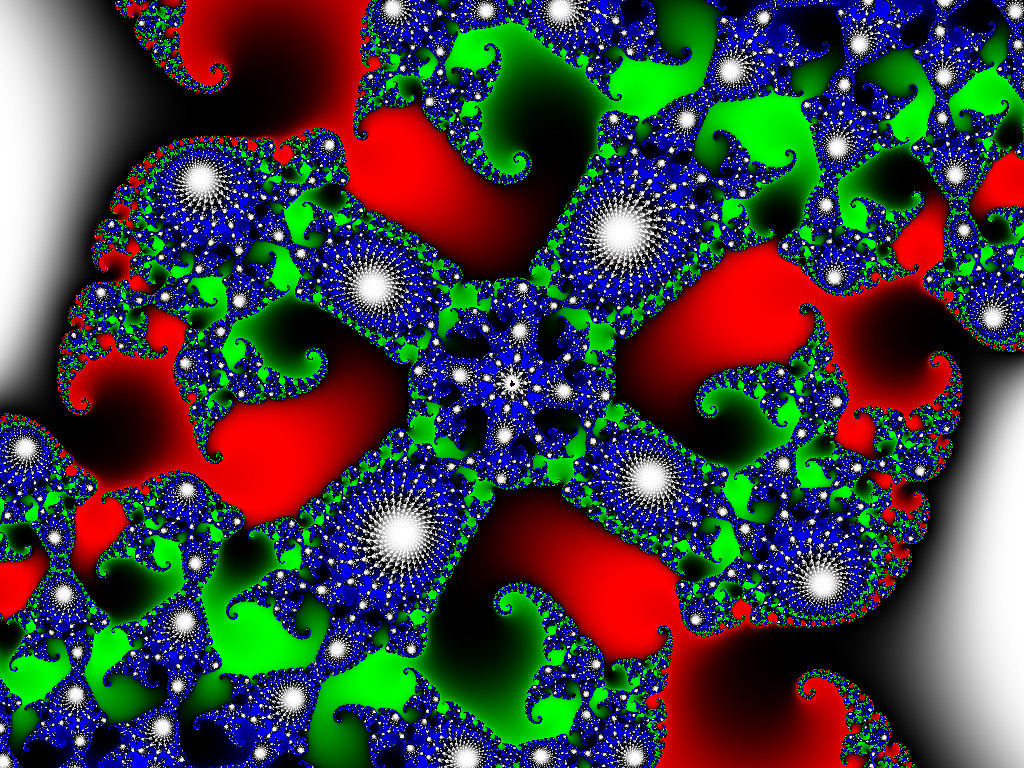
Here is another set of data, this time from the image that looks like this:

Here again we see the median filter is performing better, although the difference is subtle. First notice, as in the previous graphs, that there are fewer points at higher count numbers with the median filter. Next notice that in the range of counts around 10,000, the median filter data show much more oscillation than the mean filter data, indicating it is better able to reproduce the high-count dwell bands, rather than washing them out like the mean filter does.
If we magnify the portion of the graph from counts 6000 to 12000 and add some guide lines to each data series we can see the difference more clearly. In the graph below, the black line is a fast moving average applied to the median filter data, while the blue line is the same moving average applied to the mean filter. The spikes are a real part of the image, corresponding to different dwell bands. The median filter is better able to reproduce them at higher count numbers than the mean filter.
Selective Supersampling
Supersampling is very expensive -- it increases rendering time by at least a factor of two, and generally more like a factor of 9 or 16. One way of reducing the time needed to achieve the benefit of anti-aliasing is to select only the noisiest points for supersampling.
There are many variations on this idea, mostly based on different strategies for selecting which points to supersample. The basic plan is to measure how different each pixel is from its neighbors, and if it is more different than some threshold, it gets supersampled in a second rendering pass. Choosing how to put a number to this difference is where lies the art to selective supersampling.
Future updates to this page will have more detail on this.
Conclusions
Here is a quick summary of the main conclusions.
- The most important thing by far for effective anti-aliasing is to use a lot of oversampling points. The biggest gains are up to the first 9 to 16 (3x3 to 4x4) samples, with only a little additional benefit from going even as high as 15x15 for most images.
- The median filter is superior to the mean filter in several fundamental theoretical ways, although the differences are often subtle in actual fractal images.
- The difference between the median filter and the mean filter becomes more noticeable as the maximum count increases and in images that have many points close to a mini-set. High max-counts cause more outliers which the median filter is better able to remove. The mean filter turns these into artifactual mid-range count values.
All content Copyright by Michael Condron. All rights reserved unless otherwise noted.
You may download, save, and print a single copy for personal use only.
Music by various sources used with permission.
Please refer to individual video file credits for details.
